
The Real Cost of Redshift Warehousing
Insights From Clients and Hands-on Testing


At Twing Data, we take a holistic view of our clients’ data stacks. This requires the ability to understand, debug, and diagnose many data systems. The data warehouse is a major focus, as it can determine whether a data system meets or falls short of a company’s needs in terms of performance and budget. The pricing models of these modern warehouse solutions can be nuanced, where a misunderstanding in configuration can potentially go forever unnoticed.
In this three-part series, we’ll take a focused look at three major data warehouse solutions, Redshift, BigQuery, and Snowflake. In part one, we’ll focus on Amazon Redshift. As Amazon's flagship warehouse offering, Redshift introduced many to the possibilities of cloud-based data warehousing, but its pricing model and configuration options demand careful consideration for optimal performance and cost management.
Understanding Redshift's Pricing Model
Redshift offers a configurable pricing structure that can be as powerful as it is complex. Pricing is divided into two main components: storage and compute, with options that cater to both smaller datasets and large-scale enterprise-level use cases. Three main system options are available:
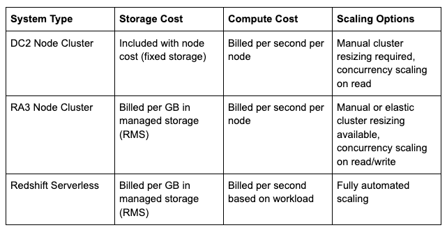
DC2 Node Cluster
Storage and compute are coupled, leading to less flexibility in system configuration and higher overhead for resizing.
The case for DC2 Nodes is increasingly harder and harder to make, as reserved RA3 instances and serverless systems better suit modern data warehousing needs (ie: high variability in compute with independently-scalable storage)
RA3 Node Cluster
The most flexible option for both regular and variable workloads, this model offers scaling by adjusting node size (elastic resizing), cluster size (node count), and number of concurrent clusters
Redshift Serverless
This is a fully-managed data system, available on demand, that automatically scales to accommodate current workloads. With no scaling or cluster uptime to manage, Serverless offers the shortest path to reliable results. While compute costs are only incurred while a workload is active, the optionality comes at a premium price not readily detectable in the docs. Lack of scaling control and the minimum charge policy (see Bonus: Death by 1000 Minimum Charges below) can result in significantly higher compute costs overall. It’s best for companies that:
Are uncertain about the cadence of their workloads
Have irregular workloads
Lack the peoplepower, technical acuity, or desire to manage an RA3 system
Coupled with the above configurations, AWS offers the option to reserve capacity for Redshift, committing to usage for a set period (e.g. 1 or 3 years) in exchange for a discounted rate. The discount scales with the length and value of the commitment, making it an attractive option for many organizations. Reserved capacity applies to various Redshift configurations, including RA3 nodes and serverless compute. However, this approach requires accurate forecasting of usage levels to maximize cost savings. For most growing companies, reserving capacity can help mitigate the resources needed for actively managing cluster uptime, while also incentivizing efficient workload distribution to optimize utilization.
Inherent Challenges with RA3
With great flexibility comes great complexity, and oversights can be costly. Redshift RA3 clusters are billed based on node size and uptime. Whether it’s at max capacity or sitting idle, AWS charges for that time. How much? That depends on the node/cluster size, as well as the number of concurrent clusters running. All options remaining equal, this essentially hinges on how fast you need data at times of peak usage. Even when factoring in the discount for reserving nodes, a persistently-running cluster with irregular heavy usage can be expensive if not closely managed. Redshift does offer a few automated or potentially-automated features to help – but be aware of a few gotchas with each:
Short Query Acceleration (SQA) - automated
Queries are classified as short or long based on a predicted runtime threshold. Short queries are prioritized, ensuring the maximum number of workloads are completed in a given timeframe
SQA Gotchas:
Prioritizing one group of queries means deprioritizing others. When execution time does not factor into the priority equation, this could lead to longer queries being perpetually deprioritized (ie: thrashing).
The threshold is dynamic by default - it changes based on machine learning using real usage. Might require experimenting with hard values.
Auto Workload Management (Auto WLM) - automated
General workload management system dynamically adjusts resource allocations within the cluster depending on current query load
Auto WLM Gotchas:
Not great for predictable, static workloads where fine-tuning resources is possible.
Requires an additional layer of management in Query Monitoring Rules (QMR), which govern the thresholds used by Auto WLM.
Critical queries that require guaranteed resources are likely hard to target using QMR.
Concurrency Scaling - automated
An additional temporary cluster is automatically provisioned to handle the overflow of queued queries during peak usage. When the overflow is handled, it shuts down. Redshift offers the first hour of concurrency scaling free, per day per cluster (this should be plenty to cover peak usage times).
Concurrency Gotchas:
If the free hour is exceeded, the concurrency scaling cluster is subject to the same per second charge, with 60-second minimum charge for each activation.
The general theme, as ever, is that the more complexity is hidden, the greater the potential sacrifice in speed and/or cost. Even concurrency scaling, which can be completely free if the system is well-optimized, can end up doubling compute costs if it’s not. Either way, tight monitoring is essential; we’ve seen situations with our customers where concurrency scaling simply stopped working without any changes to the data warehouse and complete silence from AWS.
In addition to concurrency scaling, other scaling options to be aware of involve changing the node type, size or count within the main cluster, and come in two flavors, each to be used in specific contexts:
Elastic/Classic Resize - schedulable, automation possible
Features used for adjusting node type, size, or count. Out of the box, these are either triggered manually or scheduled, but, using the API, the operation can be integrated with monitoring for full automation. Elastic is faster but more limited in terms of types of scaling possible. If elastic doesn’t serve your purpose, classic can handle more complex changes.
Resizing can be a blog topic on its own, and beyond the scope of this work. A docs link will have to suffice: https://docs.aws.amazon.com/redshift/latest/mgmt/resizing-cluster.html
Saving Data, Losing Dollars
Up to now, we haven’t touched on details around storage management. If you’re already sold on serverless, you’re in luck - storage scales 100% independently of compute and is charged per GB/month. If RA3 is more your flavor, and you have or expect to have significant amounts of data, get ready for more to manage!
RA3 nodes of different sizes have corresponding compute and storage stats. Redshift Managed Storage (RMS) capacity ranges from 1-128 TB depending on the node size. Due to the hard limits on RMS capacity, both compute and storage needs must be factored into the decision around node size/count. While storage is technically billed separately (per GB/month), these storage limits essentially manifest in a partial coupling of compute and storage billing. Maxing out the size and number of nodes in a cluster, the storage limits can reach petabyte scale. But as nodes are added and sized according to max RMS needs, uptime costs increase. Given modern companies collect increasingly more and more data, it’s no wonder solutions that completely decouple compute and storage, like Redshift Serverless or Snowflake, are so popular.
The only independent scaling solution for RA3 cluster users is to store certain data in S3 and access as needed using Redshift Spectrum. While there are cost and efficiency sacrifices compared to RMS, they are typically small if handled correctly. Here are some suggestions:
Avoid data transfer fees by storing data in the same location as your cluster
Experiment with format/compression types to determine the most efficient
Partition data by frequently-filtered columns
At Twing Data, we test your flows with various file/compression formats as part of our system optimization service.
Bonus: Death by 1000 Minimum Charges
Consider two scenarios, in which two companies with unique needs choose their systems wisely:
Scenario 1: Out of uncertainty in data system requirements, you’ve decided not to reserve your new company’s RA3 instance. But you’ve compensated by painstakingly studying, testing and optimizing its configs, and have seen significant cost savings and efficiency gain.
Scenario 2: Given your growing company’s sizable task backlog and fast-changing data needs, you decide to forgo the complexity of managing a cluster and use Redshift Serverless, which has allowed your small team to build a data system quickly while still focusing on business-critical items.
Similar to these scenarios, at Twing Data we frequently see talented teams making sound decisions validated by positive outcomes. Yet they’re still likely overpaying on their data warehouse. One reason we frequently see is Redshift’s minimum charge policy, a nasty little detail that deserves much more consideration than it usually gets. Non-reserved RA3 clusters and Serverless options both have similar per-workload and per activation minimum charge policies. To manage around them, each requires a unique approach.
Policy: 60-second minimum per activation, and charged per second of uptime after that.
RA3: Since charges are based on cluster uptime, if your instance is not reserved, it is likely because you plan on managing cluster uptime based on less-frequent, periodic access. The risk here is triggering deactivation/reactivation within a minute, causing multiple 1-minute charges in that time. If possible, designate downtimes explicitly and orchestrate workloads accordingly.
Serverless: Charges are based on resources in use only. These systems manage uptime automatically, shutting down after 1 hour of idle time. The docs are very unclear about how minimum charges apply to serverless instances, so I’ll clarify based on our experience:
The 60-second minimum charge applies to every minute in which a workload is run according to the base capacity of the instance
The per-second charge applies to the amount of seconds within the minute a certain number of RPUs (Redshift Processing Units) were used.
You are charged for at least the full billable minutes at the selected base (minimum) capacity of your instance for each minute any workload is running. It’s possible to exceed the minimum charge if capacity is scaled to meet higher demand within that minute.
Due to this policy, serverless systems are best suited for data systems that see irregular usage, as the heavy-handed minimum charge policy is offset by the lack of compute overhead when the system is idle.
Another thing to note about the serverless system is that 1 hour of idle time will trigger a deactivation event. If your company frequently goes > 1 hour without a new workload, the serverless instance will timeout. In our experience, when the system reactivates for the next workload, it introduces up to 10 seconds of latency. Remember, idle time is uncharged in a serverless setup, so it’s only a disadvantage for the instance to deactivate. We’ve seen companies avoid instance deactivation by scheduling a simple query, such as “SELECT 1;” every 55 minutes or so; it’s a simple tradeoff to pay for an occasional minute of base execution to avoid latency issues.
Takeaways
Amazon Redshift is a capable and versatile data warehouse, with options for a broad range of requirements. And, it should be noted, if already using other AWS services, the benefits of using Redshift, such as the Aurora/Redshift zero-ETL integration, are significant. However, the complexity involved in selecting, monitoring and maintaining an optimal system is high, with the potential for massive unnecessary expense. In the next part of this series, we’ll explore Google BigQuery, which takes a completely different approach to pricing and resource allocation.
For more on optimizing Redshift, we’ll soon release a breakdown between sort/dist keys and compare them with partitioning and clustering columns used by other modern cloud warehouses. Keep an eye out!
At Twing Data, we understand that no two businesses are alike, and neither are their data warehouse needs. With our expertise in query metadata analysis, organizations gain visibility into their Redshift usage patterns and the knowledge needed to make informed decisions. Reach out to learn how we can help you uncover hidden costs and turn insights into actionable savings.