The Real Cost of BigQuery

Why Serverless? Why BigQuery?

In 2017, The Economist published an article titled “The World’s Most Valuable Resource is No Longer Oil, But Data”.

As both the fuel that drives AI progress, as well as the core business of the largest companies in the world, it’s no wonder modern companies of all sizes, stages and industries implement a data strategy with a bias towards storing as much as possible, just in case. Since the hardware overhead and technical requirements of implementing and managing these systems in the traditional way put data systems out of the reach of small or agile businesses, cloud providers have emerged to fill the gap. These providers are able to leverage their scale to offer data systems affordable and accessible enough for businesses of any scale. At the pinnacle of accessibility sits the serverless model, where the provider securely distributes resources across accounts dynamically based on demand, serving them within managed environments that, to varying degrees and ways, abstract much or all of the complexity involved. In exchange, the user gets a simple way to reliably store and access their data at relatively transparent pricing.

Google Cloud’s implementation, BigQuery (which we'll shorthand as BQ), is a shining example of serverless infra. Google’s BQ documentation is robust, and while there will be some information overlap, the goal here is to add real-world usage context.

Getting Into the The Guts of BigQuery

High level, BigQuery (BQ) is a managed system that abstracts and integrates several proprietary elements, as well as many independent Google Cloud Platform (GCP) services. These elements populate, support or interact within BQ’s 2 main segments: the Data Plane and Control Plane.

• Data Plane: Encompases the storage (Colossus), compute/execution (Dremel), and networking (Jupiter) layers, which contain logic and resources for storing and reading data as well as query processing. It executes queries by reading, processing and returning data from Colossus via Dremel using allocated slots.

• Control Plane: Responsible for metadata tracking, high-level resource allocation, query parsing/validation, and job orchestration.

Here is the 50,000 ft view of the architecture at large:

It’s a complex system, but the result is the orchestration of several highly-optimized components working in sequence and parallel to dynamically handle a wide variety of conditions and applications. As this is a general overview and not a deep dive into one particular component, we’ll stick to examining 2 significant elements in the Data Plane at mid-depth.

Colossus, the underlying storage layer for several GCP services, including BQ and Google Cloud Storage (GCS), is fundamentally aligned with serverless principles; BQ’s integration with Colossus stands out by fully managing data-loss prevention with automatic multi-region data replication, at no additional cost. Within Colossus, BQ stores data in Capacitor format, their proprietary, highly-compressed columnar storage structure. This formatting is also fully managed, with no configuration options available. Additionally, a storage optimizer periodically rewrites files in a format that is more efficient for querying. The primary 2 manual storage optimizations, partitioning and clustering, which we’ll touch on later, offer some user control, but even clustering on changing data requires a layer of automated re-clustering that’s managed internally.

The pattern of highly abstracted complexity doesn’t stop at Colossus. Dremel, the query compute engine, rewrites or breaks down executed queries into stages, then enables the dynamic provisioning of very small resource units, called “slots”, in parallel for running workload stages across all existing orgs. The exact algorithm governing resource provisioning is, of course, not publicly available, but generally it’s based on a range of factors like query complexity and overall system load, and even down to a query’s particular execution stage. The goal of optimizing efficiency—and by extension, minimizing waste—is balanced against the need to ensure that some level of compute capacity remains available, even for inactive organizations (they call this “Fair Scheduling”).

With so many layers of management systems, the natural question is, 'How well does all this work?' While answering in full is beyond the scope of this section, it's largely an academic question. Users have no direct control over these internal mechanisms, aside from workload-level optimizations or switching providers. Given the sheer scale and automation of BigQuery, its performance remains a modern engineering feat, even if there are some inefficiencies.

Breaking Down BigQuery Costs: Storage and Compute

While storage and compute resources are largely automated, there are yet many ways to configure when and how they’re used.

Storage

BigQuery offers two primary pricing models, Logical and Physical Bytes Storage Billing (LBSB and PBSB respectively). Each model has a half-price long-term version as well, which is automatically set per table after 90 days without modification to the table.

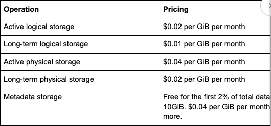
Metadata storage has quite the elaborate pricing model. That’s for good reason: the metadata is stored differently than user data because it’s accessed frequently by the system and crucial for warehouse functionality. If metadata storage begins to surpass the 2% + 10 GiB free tier threshold, it is likely an indication that there is a path to reducing metadata generation (we’ll touch on optimizations in the next section).

While not technically part of BigQuery, it’s also worth mentioning that strategically integrating GCS into BigQuery operations can enable other ways to save money on storage. Aside from handling unstructured and semistructured data storage, GCS is commonly used for storing archived data at a fraction of the cost. Most practically, GCS is ideal for staging tables due to its capacity for large-scale data ingestion, and broad support of data and compression formats. Also, hybrid pipelines can use GCS as the data bridge that connects to other storage systems.

Compute

Fully separated from storage pricing, compute pricing options range from fully on-demand to reserved capacity, or even a blend of both.

• On demand: You’re charged based on the amount of data scanned. There is no minimum usage, and the first 1 TiB per month is free. Fair scheduling reasonably ensures that each query has equal access to available slots, whether the org is highly active or mostly inactive. The resource limit for on-demand usage is 100 concurrent queries and/or 2000 slots at a time (per project per org), with 2 exceptions: the slot limit is subject to availability, and if even more are available they might be used to push through small workloads (this they call transient burst capability)

• Capacity based: In this scheme, charging is based on the amount of slots “reserved”. This reservation can be a static amount, or, optionally, a min/max range can be set to enable autoscaling for highly dynamic or unpredictable requirements. An optional 1-3 year commitment is available for Enterprise/Enterprise Plus tiers, offering discounts for committing to continuous billing for an amount of persistent compute capacity. While this ensures resource availability at all times, any autoscale compute used in addition to commitment slots are charged at the un-discounted rate. At higher volumes and commitment levels, it’s also possible to negotiate additional discounts. Finally, the pay-as-you-go option, available on all capacity-based tiers, is similar to on-demand in that charges only occur while resources are in use. One caveat here is that the set minimum reserved slots are the minimum to be used, no matter how small the workload. Another is that resources made available for a workload stay up for 60 seconds after use. With certain cadences of usage, this can be a factor worth investigating.

These pricing options can be pieced together like legos to fit your needs. Slots can be reserved per team, project, folder, or even workload type. Scaling on reserved slots can use capacity-based autoscaling or on-demand slots.

Finally, it’s worth mentioning that when these capacity-based “editions” were introduced a few years ago, they discontinued the flat-rate + flex slots model, which allowed a more deliberate or scheduled approach to reserved resource scaling. Now, even capacity-based scaling is 100% automated, further leaning away from traditional provisional models and into a fully-managed experience.

Managing a Managed System

The fully-managed services within BigQuery are highly nuanced and opinionated. Understanding how they work and what they prefer are crucial for optimizing usage. Levers like query composition, partitioning/clustering tables, metadata management and more make massive impacts on efficiency and costs. As usual, the official documentation covers optimizations fairly well, but we’ve found there’s so much nuance that even talented teams can overlook major points. I’ll drill into one peculiarity not addressed by BigQuery’s query optimizer.

Consider the following query and execution graph:

Since cte1 is referenced twice, BigQuery executed the CTE both times. Under the hood, BQ tends to treat non-recursive CTEs by inlining them in the final query plan as part of the plan creation process.

A possible optimization is to materialize the data that will be used multiple times:

Of course, this scenario is a bit contrived. And, in this simple example, while slot seconds are saved, billed bytes are equivalent. That means we get increased efficiency, but with on-demand pricing the cost doesn’t change. With increased CTE complexity, though, all metrics, including bytes processed/billed are dramatically affected in expected and unexpected ways. While it might appear obvious that reducing compute and data scanned by caching partial data as an initial step is beneficial, consolidating the entire query can help the optimizer in other ways that can offset the CTE reruns.

The high-level takeaway is that it might be worth testing significant workloads that fit this profile with temp tables.

But wait, there’s more! Temp tables in BigQuery are session-based. As long as the session is live, any temp tables created within persist. In the console, a session in this context really only means per tab, per single or multi-statement execution. But the real value is in its API usage, through what they creatively call BigQuery Sessions. A session can be generated during an API call, then referenced in subsequent API calls to associate with the same session. That means an early API call can generate temp tables and later calls can use them. Essentially, it amounts to a caching layer for larger datasets, where intermediate results remain in BigQuery instead of overloading front or back ends.

An example of this put to great use is for dashboards with multiple levels of drill downs, where complex aggregations are done at each level. Within a session, a temp table can store the data for each level, so the user can navigate down, back out, then down again with no need to wait for redundant heavy computation or rely on client-side storage.

As I said before, temp tables persist for the duration of the session. A session, if not manually terminated, will deactivate automatically after 24 hours of inactivity or 7 days after creation. Depending on the application, this can have a major impact on a system’s performance, cost efficiency, and user experience.

The TL;DR on BigQuery

BigQuery and its surrounding ecosystem is an incredible complex of intricate, interlocking systems operating at enormous scale. Every piece contains so many layers of automated management based on unknowable conditions. With almost no barriers, it really just works.

Having said that… (Curb, anyone?), to work with the system instead of against it requires a relatively deep understanding of proprietary behaviors. In a traditional warehouse, user management means to manage resources in a cluster, tuning query execution, and provisioning capacity. In BigQuery, control shifts from explicit resource management to understanding the inner workings of BigQuery’s execution model, slot allocation, caching mechanisms, and query optimizations.

We put together a similar guide for Redshift last month – you can find it here

At Twing Data, we specialize in saving clients time and money on their data systems. By analyzing warehouse metadata, our stack-agnostic product builds end to end system models based on how they’re actually used, surfacing underused resources, overlooked workload inefficiencies, suboptimal warehouse scaling, and much more.

Curious if there’s room to optimize your data spend? We’d love to take a look and share what we find—no strings attached.

Stay tuned for a deeper dive into optimizing within BigQuery.